In Search Of The Essence Of Quantum Machine Learning
How parameterized quantum circuits turn exponential Hilbert spaces into learning models
Classic machine learning already provides universal approximators and massive models. So why resort to quantum circuits? This is the search for the real challenge, namely to design problem-specific circuits that translate theoretical capacities into practical learning.
by Frank ZickertSeptember 2, 2025
What could Quantum Computing is a different kind of computation that builds upon the phenomena of Quantum Mechanics. offer that would justify the effort involved in establishing the new field of Quantum Machine Learning is the field of research that combines principles from Quantum Computing is a different kind of computation that builds upon the phenomena of Quantum Mechanics. with traditional Machine Learning is an approach on solving problems by deriving the rules from data instead of explicitly programming. to solve complex problems more efficiently than classical approaches. The bar is set high. Over the past decade, classical Machine Learning is an approach on solving problems by deriving the rules from data instead of explicitly programming. has achieved remarkable results. Transfomer now capture far-reaching dependencies in texts with more than billion parameters. Their results—texts, source code, images, even videos—are often indistinguishable from human work.
Figure 1 Generative AI creates an image of generative AI... created by generative AI
And that's only one part of it. Classic Machine Learning is an approach on solving problems by deriving the rules from data instead of explicitly programming. encompasses much more than Generative Artificial Intelligence. An artificial neural network is a computational model of interconnected nodes inspired by biological neurons, used to approximate functions and recognize patterns. are universal function approximators: with sufficient capacity, they can represent any continuous function. Kernel is... map data to high-dimensional Hilbert Space where linear separation is possible. Optimization is... algorithms such as Stochastic Gradient Descent and Adam can be reliably scaled to millions or billions of parameters. Together, these advances form an arsenal of techniques that dominate tasks in the fields of image processing, language, and structured data alike.
Against this backdrop, we must critically examine the core approach of Quantum Machine Learning is the field of research that combines principles from Quantum Computing is a different kind of computation that builds upon the phenomena of Quantum Mechanics. with traditional Machine Learning is an approach on solving problems by deriving the rules from data instead of explicitly programming. to solve complex problems more efficiently than classical approaches. , which focuses on a A parameterized quantum circuit (PQC) is a Quantum Circuit whose Quantum Gate depend on adjustable Real Number parameters. These parameters are optimized by a classical algorithm to minimize a Cost Function making parameterized quantum circuits the central building block of variational quantum algorithms. They serve as an interface between Quantum Computer and Optimization is... tasks, connecting abstract algorithm design with practical implementation. as a Model is.... The Quantum Circuit is trained A Variational Quantum Algorithm is a hybrid quantum–classical algorithm in which a Quantum Circuit is paramterized by a classical routine. This means, it usually computes the values for rotation angles used inside this A parameterized quantum circuit (PQC) is a Quantum Circuit whose Quantum Gate depend on adjustable Real Number parameters. These parameters are optimized by a classical algorithm to minimize a Cost Function making parameterized quantum circuits the central building block of variational quantum algorithms. They serve as an interface between Quantum Computer and Optimization is... tasks, connecting abstract algorithm design with practical implementation. during a classical pre-processing step. Additionally, the measurement results are interpreted during a classical post-processing. and its parameters are updated through a classical Optimization is... loop. This design turns the A parameterized quantum circuit (PQC) is a Quantum Circuit whose Quantum Gate depend on adjustable Real Number parameters. These parameters are optimized by a classical algorithm to minimize a Cost Function making parameterized quantum circuits the central building block of variational quantum algorithms. They serve as an interface between Quantum Computer and Optimization is... tasks, connecting abstract algorithm design with practical implementation. itself into a function approximator that competes directly with An artificial neural network is a computational model of interconnected nodes inspired by biological neurons, used to approximate functions and recognize patterns., Kernel is..., and other classical architectures.
For such an approach to be viable, a A parameterized quantum circuit (PQC) is a Quantum Circuit whose Quantum Gate depend on adjustable Real Number parameters. These parameters are optimized by a classical algorithm to minimize a Cost Function making parameterized quantum circuits the central building block of variational quantum algorithms. They serve as an interface between Quantum Computer and Optimization is... tasks, connecting abstract algorithm design with practical implementation. must offer some representation capacity or computational efficiency that goes beyond what these established Model is... already achieve. Without this, they run the risk of becoming expensive imitations of methods that already work, and the rationale for Quantum Machine Learning is the field of research that combines principles from Quantum Computing is a different kind of computation that builds upon the phenomena of Quantum Mechanics. with traditional Machine Learning is an approach on solving problems by deriving the rules from data instead of explicitly programming. to solve complex problems more efficiently than classical approaches. disappears.
So what does a A quantum algorithm is a step-by-step computational procedure designed to run on a quantum computer, exploiting quantum phenomena such as superposition, entanglement, and interference to solve certain problems more efficiently than classical algorithms. offer that a classical algorithm does not? The first real clue comes from comparing how classical and quantum Model is... expand data. In a classical Model is..., an input Vector is assigned to a Feature Space. In this space, the number of Basis State grows polynomially (usually linearly) with the dimension .
A quantum Model is..., on the other hand, embeds an input into the state space of qubits. This state is a Superposition is... of all computational Basis State. Instead of a polynomially growing set of features, the Quantum Circuit opens up access to an exponentially large basis. Each A qubit is the basic unit of quantum information, representing a superposition of 0 and 1 states. doubles the number of accessible states, creating a representation landscape that no classical Model is... can efficiently match.
Figure 3 Growth of state space, note the y-axis scaling
This shift puts the problem in a new context. The promising potential of A parameterized quantum circuit (PQC) is a Quantum Circuit whose Quantum Gate depend on adjustable Real Number parameters. These parameters are optimized by a classical algorithm to minimize a Cost Function making parameterized quantum circuits the central building block of variational quantum algorithms. They serve as an interface between Quantum Computer and Optimization is... tasks, connecting abstract algorithm design with practical implementation. lies not in marginal improvements, but in the fact that they open up a Feature Space whose size grows exponentially with the number of A qubit is the basic unit of quantum information, representing a superposition of 0 and 1 states.. This exponential expansion is the structural reason for assuming that a quantum Model is... could offer an advantage for Machine Learning is an approach on solving problems by deriving the rules from data instead of explicitly programming. .
However, access to a Hilbert Space of dimension is meaningless if the Model is... does not use it. A quantum Kernel is... must do more than embed inputs in a huge space. It must use this space in such a way that a separation is achieved that cannot be achieved with any efficient classical construction.
Figure 4 Naive use of technology does not exploit its full potential.
So even though we know that capacity is exponential, when we use naive Encoding we fall back on forms that also classical Kernel is... can approximate, too. Any possible Quantum Advantage vanishes. The unresolved problem therefore lies in finding out how data Embedding and algorithms can be designed that actually make use of the exponential structure. Until then, the exponentially growing Hilbert Space remains a theoretical promise rather than a practical advantage.
Fortunately, Quantum Machine Learning is the field of research that combines principles from Quantum Computing is a different kind of computation that builds upon the phenomena of Quantum Mechanics. with traditional Machine Learning is an approach on solving problems by deriving the rules from data instead of explicitly programming. to solve complex problems more efficiently than classical approaches. is an active area of research. And there is a number of publications that show how access to an exponentially large Hilbert Space.
Yet, unfortunately, that research is not precisely beginner-friendly. Because the articles sound something like this:
Define the Quantum Feature Map is... and the associated quantum Kernel is... as the Quantum State Overlap
For any positive semidefinite Kernel is..., there exists a unique Reproducing Kernel Hilbert Space of functions with Inner Product, characterized by the reproducing property:
In the case of , the Reproducing Kernel Hilbert Space is the closure of finite linear combinations of the quantum features . Havlicek, V., 2019, Nature, Vol. 567, pp. 209-212 show that for certain Encoding, constructed from commuting Quantum Circuit approximating the Kernel is...
to additive error is classically hard on average, unless the Polynomial Hierarchy collapses. Thus, while Kernel is... values can be efficiently estimated on a Quantum Computer, they are conjectured to be intractable to approximate classically.
Consequently, the Reproducing Kernel Hilbert Space is computationally accessible only with quantum resources, establishing a separation in computational expressivity between quantum and classical kernel methods.
The findings in the literature are rigorous, but not always practical. They prove that certain Quantum Kernel are difficult to approximate classically. Yet, they do not explain how to develop working models for real data sets. There are two main challenges here.
Challenge 1: Choosing useful encodings
It is easy to write a function with the corresponding kernel . The difficult part is designing so that the kernel does two things at once:
captures the structure of the actual learning problem and
remains provably hard to approximate classically, while still being trainable on real quantum hardware.
McClean, J.R., 2018, Nature Communications, Vol. 9, pp. 4812 In this setting, Gradient disappear exponentially fast with the number of A qubit is the basic unit of quantum information, representing a superposition of 0 and 1 states., a problem known as Barren Plateau. This makesOptimization is... practically impossible without additional structure or careful initialization.
Therefore, it is not enough to simply place a model in the vast Hilbert Space. But the Quantum Circuit architecture must be chosen in such a way that learning remains possible.
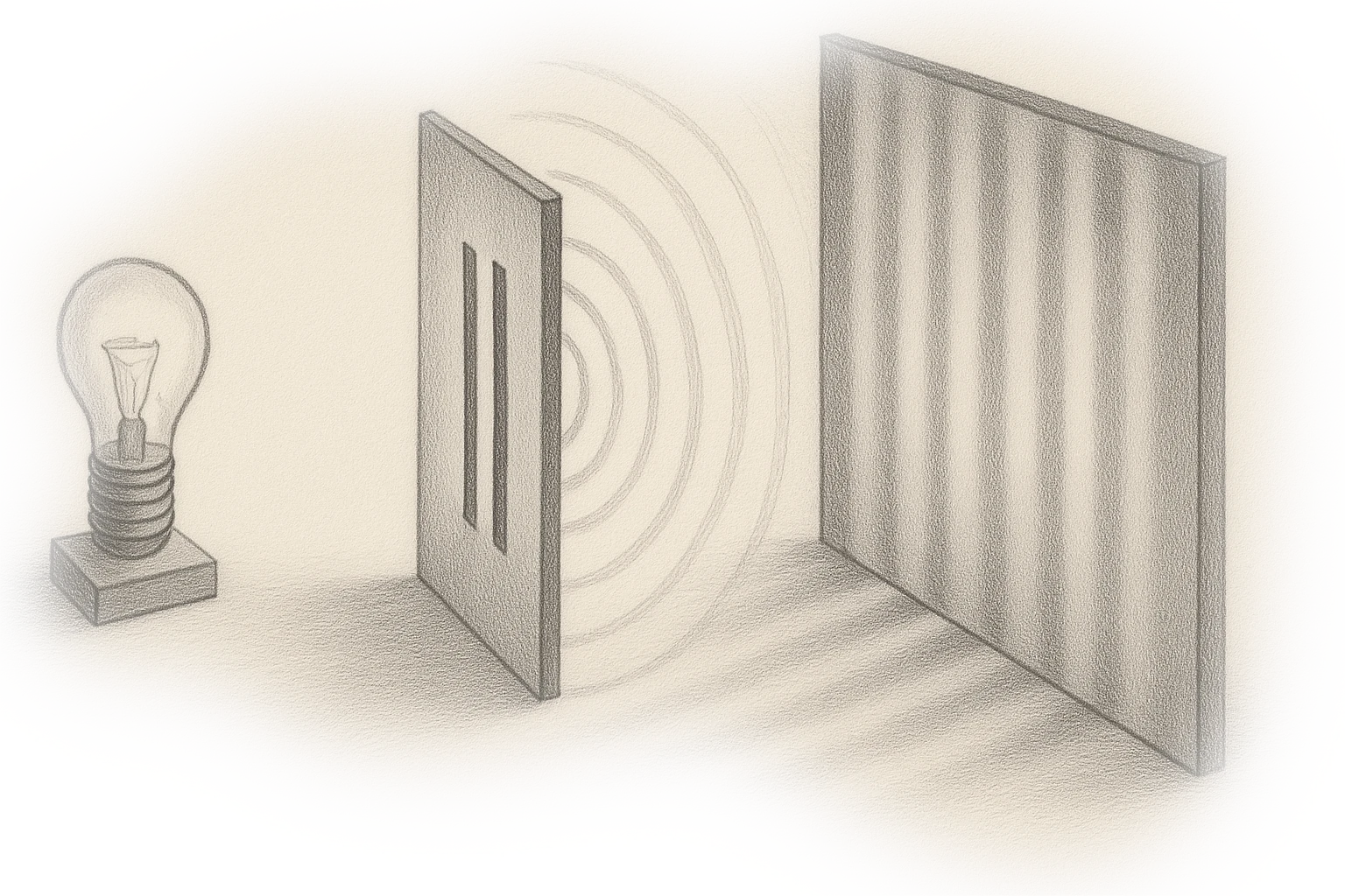
Figure 5 The double-slit experiment
The key mechanism for accessing the exponential Hilbert Space is Interference is.... When a Quantum Circuit is running, the system Unitary evolution is the reversible, deterministic time evolution of a quantum system governed by a unitary operator. into a Superposition is... of many computational paths. Each path contributes a Amplitude and the probability of an outcome depends on the square of the sum of these Amplitude.
By tuning the Quantum Gate parameters, you change how the paths reinforce or cancel each other out. This selective Interference is... allows the Quantum Circuit to highlight certain patterns in the input and suppress others. The effect is a Decision Boundary that can be highly nonlinear and structured. In classical Model is... capturing the same pattern would often require deep An artificial neural network is a computational model of interconnected nodes inspired by biological neurons, used to approximate functions and recognize patterns. or a large number of parameters.
In physics, the Double Slit shows how a particle's probability distribution depends on constructive and destructive Interference is... of two possible paths. In circuit form, the same effect is created with just three gates:
A Hadamard Operator puts the A qubit is the basic unit of quantum information, representing a superposition of 0 and 1 states. into a Superposition is... of is a basis state. and is a basis state..
A rotation around the -axis, , introduces a Quantum Phase that depends on the input data .
A second Hadamard Operator brings the two paths back together so that their AmplitudeInterference is....
The resulting probability of measuring outcome is then
while outcome occurs with probability
As you can see, both probabilities depend on the sine and cosine of the specified rotation around the -axis that determines the Quantum Phase.
This explanation is quite mathematical. It's more than time to make the principle tangible and look at it in practical terms.
The following listing depicts the core of the circuit implementation in Qiskit.
double_slit.py
1
2
3
4
5
6
7
8
9
10
11
defdouble_slit_single_qubit():
qr = QuantumRegister(1, "qr")
cr = ClassicalRegister(1, "cr")
theta = Parameter("theta")
qc = QuantumCircuit(qr, cr, name="double_slit")
qc.h(qr[0])
qc.rz(theta, qr[0])
qc.h(qr[0])
qc.measure(qr[0], cr[0])
return qc, theta
We define a quantum circuit with two registers.
defines a quantum register with a single A qubit is the basic unit of quantum information, representing a superposition of 0 and 1 states..
defines a classical register with one classical bit to store the measurement outcome.
We add three Quantum Gate and a Measurement to our circuit:
The puts the A qubit is the basic unit of quantum information, representing a superposition of 0 and 1 states. into a Superposition is... state in which the Amplitude of both Basis State are equal. In other words, if we were to measure this Quantum State is..., we would measure and with the same probability.
The applies a rotation around the -axis by the angle that we take as an external parameter . This means, it is not yet fixed at a certain value but is specified when we use the quantum circuit. The rotation does not affect the measurement probability of either Basis State. But it changes the Quantum Phase of is a basis state..
The moves the Quantum State Vector away from a Superposition is... state in which both Basis State have an Amplitude of the same size. Depending on the Quantum Phase applied, it moves either in the direction of is a basis state. or in the direction of is a basis state..
The final measures the qubit in the Computational Basis and puts the result into the classical register cr.
This function the quantum circuit qc and the parameter theta.
If you look at the mathematical explanation of our circuit again, you will see that we do not feed ("theta") directly into the - operator, but rather . This a function ("phi") of .
This function serves as a feature mapping that translates the external variable into the actual gate angle used in the circuit. It implements a simple linear transformation:
where controls how many oscillations of the Interference is... pattern occur over the interval . introduces a phase shift along the -axis.
This mapping ensures that the measurement probabilities and exhibit the characteristic sinusoidal patterns associated with the Interference is... of individual A qubit is the basic unit of quantum information, representing a superposition of 0 and 1 states., with adjustable frequency and phase shift. These parameters and are optional and are therefore sometimes omitted for the sake of conciseness.
The corresponding function in Python is straightforward:
double_slit.py
1
2
3
defphi(x, w=1.0, b=0.0):
# Data-to-phase map: phi(x) = w * x + b
returnfloat(w * x + b)
In the next step, we use our double_slit circuit.
double_slit.py
1
2
3
4
5
6
7
8
9
10
11
12
13
qc, theta = double_slit_single_qubit()
x = pi
val = phi(x, w=3.0, b=0.6)
bound = qc.assign_parameters({theta: val})
simulator = Aer.get_backend("aer_simulator")
result = simulator.run(bound, shots=1_000).result()
We start with a Classical Preprocessing, we create the actual circuit to be executed.
We and obtain its instance and an instance of the parameter theta.
We spcify and map it into a circuit parameter through the feature map phi. This step turns classical data into a phase angle. With w=3.0, we specify to pack three oscillations into the range between and . Further, we specify the starting offset to be b=0.1.
Next the symbolic placeholder . This makes the circuit concrete: when executed, it rotates exactly by this phase. Without this binding, the circuit is just a template.
In the next block, we run the quantum circuit. In our case, a localQuantum Simulation will do.
We specify an ,
times,
,
and of measuring the qubit as either or .
Finally, we .
The following listing depicts the measurement output.
As we can see, our empiric results are close to the calculated theoretical values.
Before you try all the different values for manually, let's write a brief convenience function to do that for us. When we run our circuit in a loop for x in np.linspace(0, 2*np.pi, 50), we get points between and .
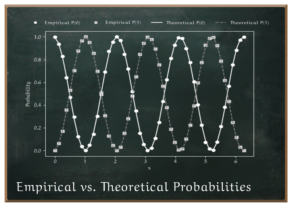
The following figure shows the plotted empirical results along the calculated theoretial values.
Figure 6 The results of the quantum circuit
The output of the double-slit circuit is not a linear threshold but a smooth, periodic curve. The measurement probability oscillates (here times) as a cosine squared of the input phase. That periodicity is the direct result of Interference is... between the two computational paths.
To mimic this behavior in a classical Model is..., you would need to generate the same sinusoidal dependence on the input. That is why, when comparing to a feedforward An artificial neural network is a computational model of interconnected nodes inspired by biological neurons, used to approximate functions and recognize patterns., the relevant question becomes: how well can it approximate functions like ? A ReLU network can only generate piecewise linear functions, so approximating a smooth periodic curve like requires hidden units to reach accuracy . The quantum circuit does it with depth and one parameter.
The circuit in Qiskit is minimal. But it impressively shows how Interference is... patterns encode input-dependent Decision Boundary. It is the most direct method to see how A parameterized quantum circuit (PQC) is a Quantum Circuit whose Quantum Gate depend on adjustable Real Number parameters. These parameters are optimized by a classical algorithm to minimize a Cost Function making parameterized quantum circuits the central building block of variational quantum algorithms. They serve as an interface between Quantum Computer and Optimization is... tasks, connecting abstract algorithm design with practical implementation. use Superposition is... and Interference is... to convert Quantum Phase information into a nonlinear classification signal.
A parameterized quantum circuit (PQC) is a Quantum Circuit whose Quantum Gate depend on adjustable Real Number parameters. These parameters are optimized by a classical algorithm to minimize a Cost Function making parameterized quantum circuits the central building block of variational quantum algorithms. They serve as an interface between Quantum Computer and Optimization is... tasks, connecting abstract algorithm design with practical implementation. do not strive for general universality. They target specific structures that are costly for classical Model is..., such as periodic decision boundaries. Therefore, Quantum Circuit are precise tools that are valuable not everywhere, but precisely where classical methods are oversized in scope and depth.
The big challenge in Quantum Machine Learning is the field of research that combines principles from Quantum Computing is a different kind of computation that builds upon the phenomena of Quantum Mechanics. with traditional Machine Learning is an approach on solving problems by deriving the rules from data instead of explicitly programming. to solve complex problems more efficiently than classical approaches. lies not in pure expressiveness, but in modeling. A A parameterized quantum circuit (PQC) is a Quantum Circuit whose Quantum Gate depend on adjustable Real Number parameters. These parameters are optimized by a classical algorithm to minimize a Cost Function making parameterized quantum circuits the central building block of variational quantum algorithms. They serve as an interface between Quantum Computer and Optimization is... tasks, connecting abstract algorithm design with practical implementation. has exponential capacity, but this capacity is useless if it is not shaped by the structure of the learning task. Just as with classical Kernel is... methods, the effectiveness of a quantum kernel or A parameterized quantum circuit (PQC) is a Quantum Circuit whose Quantum Gate depend on adjustable Real Number parameters. These parameters are optimized by a classical algorithm to minimize a Cost Function making parameterized quantum circuits the central building block of variational quantum algorithms. They serve as an interface between Quantum Computer and Optimization is... tasks, connecting abstract algorithm design with practical implementation. depends on the problem domain. A useful model must exploit quantum correlations in a way that is tailored to the specific structure of the task.
Progress is achieved through architectures and training methods tailored to real-world problems, not by striving for larger Hilbert Space. The advantage of Quantum Circuit will only be realized if they are developed to solve specific learning tasks and not to demonstrate Quantum mechanics is the branch of physics that describes the behavior of matter and energy at atomic and subatomic scales..